Responsible AI: Interpret-Text with the Classical Text Explainer

In the previous post you got an overview about interpretability, and the different explainers available in the Interpret-Text tool. In this post you will get an understanding of how to use one of the explainers: Classical Text Explainer.

The Classical Text Explainer is an interpretability technique used on classical machine learning models, and covers the whole pipeline including text pre-processing, encoding, training and hyperparameter tuning, all behind the scenes.

For pre-processing it uses a bag-of-words encoder and logistic regression for training as a default configuration.

As an input model, Classical Text Explainer supports two model families: scikit-learn linear models (coefs_ call) and tree-based models (feature_importances call). Additionally, any models with similar layout and suitability for sparse representation can be used soon.

The API enables users to extend or move around the different modules such as the pre-processor, the tokenizer, or the model, and the explainer still can pull in and use the tools implemented in the package together with your configuration.

By reading this post, you get an overview about how to use the explainer, and you will understand how the model works and what is the meaning of the results of the different measures.

Setting up the environment

To follow the tutorial, please install Anaconda with Python 3.7, and open Anaconda Prompt. This can be done on a computer locally, or on a virtual machine. Get the repository to get started and move to the folder that is created.

git clone https://github.com/interpretml/interpret-text.git
cd interpret-text

The next step is to prepare the environment to include all the necessary packages.

For CPU:
python tools/generate_conda_files.py
conda env create -n interpret_cpu --file=interpret_cpu.yaml
conda activate interpret_cpu

For GPU:
python tools/generate_conda_files.py --gpu
conda env create -n interpret_gpu --file=interpret_gpu.yaml
conda activate interpret_gpu

Python packages need to be installed as well together with a widget that is required for dashboarding.

cd python
pip install -e .
jupyter nbextension install interpret_text.experimental.widget --py --sys-prefix
jupyter nbextension enable interpret_text.experimental.widget --py --sys-prefix

And finally install the notebook where the Python code will run, then start the notebook in your favorite browser.

cd..
pip install notebook
jupyter notebook

The environment now should look something like this:

Implementation

Create a new notebook with Python 3, by using the NEW button on the top right corner of the screen. The user should see an environment similarly like on the picture below.

The Notebook environment and the working directory is defined with the following code snippet. Do not forget about using matplotlib, otherwise some graphics might not work perfectly.

%matplotlib inline

import sys
import os
sys.path.append("../..")

The next step is to import the dataset for training, using a predefined function that extracts the data and builds a Pandas Dataframe which is now ready to use.

from notebooks.test_utils.utils_mnli import load_mnli_pandas_df

df = load_mnli_pandas_df("./temp", "train")
df = df[df["gold_label"] == "neutral"]

X_str = df['sentence1']
ylabels = df['genre']

Here is a fragment of the dataset, showing the labels (genre) and the features (sentence1).

df[["genre", "sentence1"]].head()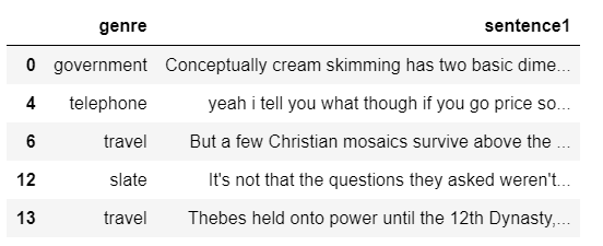

It is a good idea to have a balanced dataset, to provide the same amount of examples for each labels before training, otherwise the training result will also be skewed.

df["genre"].value_counts()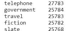

It is now visible that the data is sort of balanced, let’s use this for training. As mentioned above, the ClassicalTextExplainer takes care of the entire pipeline, and the LabelEncoder of sklearn is going to be used for text pre-processing.

from interpret_text.experimental.classical import ClassicalTextExplainer
from sklearn.preprocessing import LabelEncoder

explainer = ClassicalTextExplainer()
label_encoder = LabelEncoder()

It is time to prepare the dataset for training and testing (104720 rows of features and layers), using the splitting function of sklearn and the LabelEncoder.

from sklearn.model_selection import train_test_split

X_train, X_test, y_train, y_test = train_test_split(X_str, ylabels, train_size=0.8, test_size=0.2)
y_train = label_encoder.fit_transform(y_train)
y_test = label_encoder.transform(y_test)

print("X_train shape =" + str(X_train.shape))
print("y_train shape =" + str(y_train.shape))

The fit function of the explainer is available to train the machine that returns the classifier results and the best parameters. The aim of the classifier is to predict the genre of the different sentences.

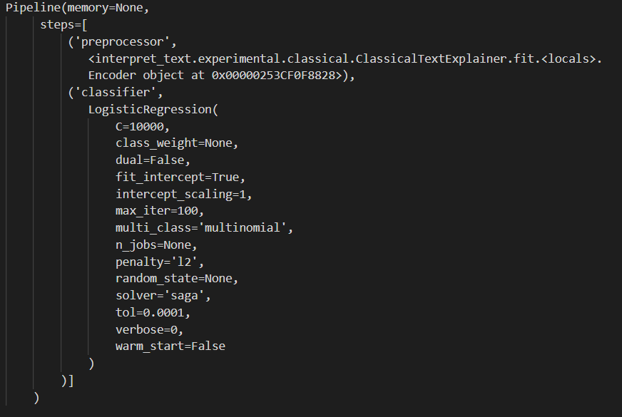
classifier, best_params = explainer.fit(X_train, y_train)

The pipeline configuration includes the preprocessor and the classifier as well, with the default LogisticRegression model and the most important parameters are chosen from this list. Remember, the specification built from these parameters works well only on this dataset and model that are defined for this article, but might not perform on the same way with a different configuration.

With the use of the test dataset, the labels now can be predicted. As a result, the accuracy, the precision, the recall and the fscore can be reviewed.

from sklearn.metrics import precision_recall_fscore_support

mean_accuracy = classifier.score(X_test, y_test, sample_weight=None)
y_pred = classifier.predict(X_test)
[precision, recall, fscore, support] = precision_recall_fscore_support(y_test, y_pred,average='macro')

print("accuracy = " + str(mean_accuracy * 100))
print("precision = " + str(precision * 100))
print("recall = " + str(recall * 100))
print("fscore = " + str(fscore * 100))

To understand these measures, it is good to know how the confusion matrix works, since from these parameters we can calculate accuracy, precision, recall and F1 score. Accuracy shows the total correctly predicted observations out of all the observations. The precision shows the correctly predicted positive observations out of all the positive observations. Recall is calculated from the correctly predicted positive observations, when it is an actual positive class. Finally, the F1 score is calculated from recall and precision, it is these two measures’ average with a weight.

But how a model can figure all this out? How does it choose the important ones from the features?

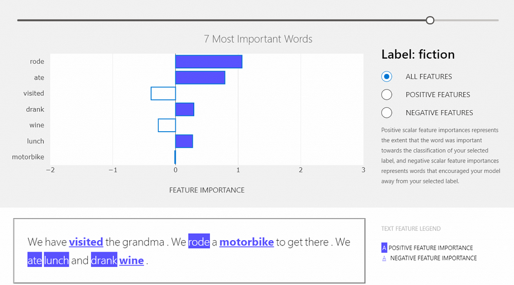
Let’s test our model with some real data, the document for this demo is going to be 3 individual sentences. The label list — that the model should choose from during prediction — is going to be the same that we used for training. The explainer should return the top feature identifiers for the selected labels.

document = "We have visited the grandma. We rode a motorbike to get there. We ate lunch and drank wine."

explainer.preprocessor.labelEncoder = label_encoder
local_explanation = explainer.explain_local(document)

A list element from a test dataset can also be passed to the explainer which would look like this:

local_explanation = explainer.explain_local(X_str[0])

To see which words are important, the explainer would rank them, and the information can be gathered with the following code:

words = local_explanation.get_ranked_local_names()
values = local_explanation.get_ranked_local_values()

The result would show the important words (words: more interesting ones are in the beginning of the list), and the values define how important that particular word is (values: same order as the words list).

Dashboard

It is really not easy to understand the result when you look at numbers only, so the visual dashboard in this case is quite handy. This is an interactive widget that shows whether the specific word has an effect on the prediction (positive features) or not (negative features). To generate and view this dashboard, run the following code.

from interpret_text.experimental.widget import ExplanationDashboard
ExplanationDashboard(local_explanation)

With the slider on the top of the dashboard, the number of important features shown can be set. On the right side, the user can see the label given to the provided document. Under this, the user can choose to see all the features or only the positive or the negative ones. By hovering on the bars in the graph, the user can see the importance values.

Conclusion

With the use of the Classical Text Explainer it is quite smooth and quick to put together a training pipeline, and the evaluation of the model is more straightforward and understandable. Users get a good overview of how the model uses the data that is provided, which allows them to improve the pipeline easier. In this post we learned about the explainer, built a training pipeline and after evaluation, generated a dashboard to understand, which words have an impact on the predicted label.

Continue the experimentation with other explainers:

• Unified Information Explainer
• Introspect Rationale Explainer

Contribution:

GitHub: Interpret-Text