Responsible AI: Interpret-Text with the Unified Information Explainer

In the previous post you got an overview about interpretability, and the different explainers available in the Interpret-Text tool. 
In this post you will get an understanding of how to use one of the explainers: Unified Information Explainer.

The Unified Information Explainer can be used when a unified and intelligible explanation is needed about the transformer, pooler and classification layers of a particular deep natural language processing (NLP) model.

Text pre-processing is handled by the explainer, sentences are tokenized by the BERT Tokenizer. At the time of writing the article, the developer must provide Unified Information Explainer a trained or fine-tuned Bidirectional Encoder Representations from Transformers (BERT) model with samples of trained data. Support for Recurrent Neural Network (RNN) and Long short-term memory (LSTM) is also going to be implemented in the future.

By reading this post, you get an overview about how to use the explainer, and you will understand how the model works and what is the meaning of the results of the different measures.

Setting up the environment

To follow the tutorial, please install Anaconda with Python 3.7, and open Anaconda Prompt. This can be done on a computer locally, or on a virtual machine. Get the repository to get started and move to the folder that is created.

git clone https://github.com/interpretml/interpret-text.git
cd interpret-text

The next step is to prepare the environment to include all the necessary packages.

For CPU:
python tools/generate_conda_files.py
conda env create -n interpret_cpu --file=interpret_cpu.yaml
conda activate interpret_cpu

For GPU:
python tools/generate_conda_files.py --gpu
conda env create -n interpret_gpu --file=interpret_gpu.yaml
conda activate interpret_gpu

Python packages need to be installed as well together with a widget that is required for dashboarding.

cd pythonpip install -e .
jupyter nbextension install interpret_text.experimental.widget --py --sys-prefix
jupyter nbextension enable interpret_text.experimental.widget --py --sys-prefix

And finally install the notebook where the Python code will run, then start the notebook in your favorite browser.

cd..
pip install notebook
jupyter notebook

The environment now should look something like this:

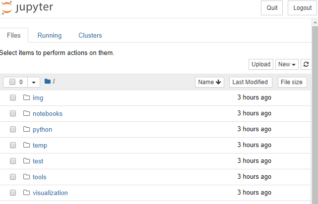
Implementation

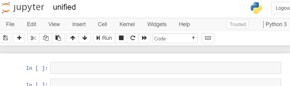
Create a new notebook with Python 3, by using the NEW button on the top right corner of the screen. The user should see an environment like on the picture below.

The Notebook environment and the working directory is defined with the following code snippet. Do not forget about using matplotlib, otherwise some graphics might not work perfectly.

%matplotlib inline

import sys
import os
sys.path.append("../..")

Some variables are defined here that will be used for training. It is possible to decrease the runtime, by setting the QUICK RUN to True. Note that doing so will affect the performance of the model. Additionally, the batch size can be set based on the configuration of the device, where the training would run. Use the is_available() function of PyTorch.

QUICK_RUN = True

TRAIN_DATA_FRACTION = 1
TEST_DATA_FRACTION = 1
NUM_EPOCHS = 1

if QUICK_RUN:
    TRAIN_DATA_FRACTION = 0.001
    TEST_DATA_FRACTION = 0.001
    NUM_EPOCHS = 1

import torch
import torch.nn as nn
    
if torch.cuda.is_available():
    BATCH_SIZE = 1
else:
    BATCH_SIZE = 9

The next step is to import the dataset for training, using a predefined function that extracts the data and builds a Pandas Dataframe which is now ready to use.

import pandas as pd
from notebooks.test_utils.utils_mnli import load_mnli_pandas_df

df = load_mnli_pandas_df("./temp", "train")
df = df[df["gold_label"]=="neutral"]

Here is a fragment of the dataset, showing the labels (genre) and the features (sentence1).

df[["genre", "sentence1"]].head()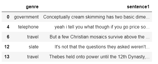

It is a good idea to have a balanced dataset, to provide the same amount of examples for each labels before training, otherwise the training result will also be skewed.

df["genre"].value_counts()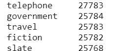

It is now visible that the data is sort of balanced, let’s use this for training. The data now is going to be splitted with the use of the train_test_split() function, and the LabelEncoder of sklearn is going to be used for text pre-processing. If the QUICK RUN is True, it is possible to pass only a fragment of the entire dataset, but this will maybe reduce the performance of the model.

from sklearn.preprocessing import LabelEncoder
from sklearn.model_selection import train_test_split
import numpy as np

#split data
df_train, df_test = train_test_split(df, train_size = 0.6, random_state=0)
df_train = df_train.reset_index(drop=True)
df_test = df_test.reset_index(drop=True)

if QUICK_RUN:
    df_train = df_train.sample(frac=TRAIN_DATA_FRACTION).reset_index(drop=True)
    df_test = df_test.sample(frac=TEST_DATA_FRACTION).reset_index(drop=True)

# encode labels
label_encoder = LabelEncoder()
labels_train = label_encoder.fit_transform(df_train["genre"])
labels_test = label_encoder.transform(df_test["genre"])

num_labels = len(np.unique(labels_train))
print("Number of unique labels: {}".format(num_labels))
print("Number of training examples: {}".format(df_train.shape[0]))
print("Number of testing examples: {}".format(df_test.shape[0]))

After the transformation, the number of training and testing features together with the label is returned. Before passing the data to the model for training, it has to be prepared by tokenizing. For this task, the BERT Tokenizer can be used for both the training and testing datasets. After this processing step, the model will receive the data as a list of tokens.

from interpret_text.experimental.common.utils_bert import Language, Tokenizer

BERT_CACHE_DIR = "./temp"

LANGUAGE = Language.ENGLISH
tokenizer = Tokenizer(LANGUAGE, to_lower=True, cache_dir=BERT_CACHE_DIR)

tokens_train = tokenizer.tokenize(list(df_train["sentence1"]))
tokens_test = tokenizer.tokenize(list(df_test["sentence1"]))

In the following two lines some extra pre-processing is done, such as specifying the beginning and the end of a sentence, the token length (MAX_LEN: change this if you want to decrease the training process’ length). Find more information about BERT implementation here.

MAX_LEN = 150

tokens_train, mask_train, _ = tokenizer.preprocess_classification_tokens(tokens_train, MAX_LEN)
tokens_test, mask_test, _ = tokenizer.preprocess_classification_tokens(tokens_test, MAX_LEN)

The next step is to load the pre-trained BERT model with the use of a sequence classifier, specifying the number of labels and the language.

from interpret_text.experimental.common.utils_bert import BERTSequenceClassifier

classifier = BERTSequenceClassifier(language=LANGUAGE, num_labels=num_labels, cache_dir=BERT_CACHE_DIR)

With the use of the training dataset, let’s start training the classifier. The aim of the classifier is to predict the genre of the different sentences.

from interpret_text.experimental.common.timer import Timer

with Timer() as t:
    classifier.fit(token_ids=tokens_train,
                    input_mask=mask_train,
                    labels=labels_train,    
                    num_epochs=NUM_EPOCHS,
                    batch_size=BATCH_SIZE,    
                    verbose=True)

print("[Training time: {:.3f} hrs]".format(t.interval / 3600))

We train the classifier using the training set. This step also involves fine-tuning the BERT Transformer and learning a linear classification layer on top of that. The classifier is now ready to score the test dataset.

preds = classifier.predict(token_ids=tokens_test, 
                           input_mask=mask_test, 
                           batch_size=512)

It is now time to evaluate the model, and review the accuracy, precision, recall and F1 score for each labels. To understand these measures, it is good to know how the confusion matrix works, since from these parameters we can calculate accuracy, precision, recall and F1 score. Accuracy shows the total correctly predicted observations out of all the observations. The precision shows the correctly predicted positive observations out of all the positive observations. Recall is calculated from the correctly predicted positive observations, when it is an actual positive class. Finally, the F1 score is calculated from recall and precision, it is these two measures’ average with a weight.

from sklearn.metrics import classification_report, accuracy_score
import json

report = classification_report(labels_test, preds, target_names=label_encoder.classes_, output_dict=True) 
accuracy = accuracy_score(labels_test, preds)
print("accuracy: {}".format(accuracy))
print(json.dumps(report, indent=4, sort_keys=True))

It is very important to understand what happens behind the scenes, how the model decides based on the different words, which label to assign to the sentence. The following code for example would return the configuration details for each layers of the classification model.

device = torch.device("cpu" if not torch.cuda.is_available() else "cuda")

classifier.model.to(device)

for param in classifier.model.parameters():
    param.requires_grad = False

classifier.model.eval()

The result should look something similar to the one on the following picture.

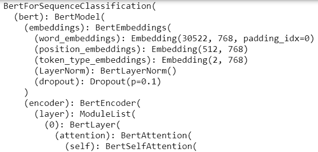
To get an explanation of the model, the Unified Information Explainer needs to be initialized by passing the model, a dataset, the CUDA device and the target BERT layer.

from interpret_text.experimental.unified_information import UnifiedInformationExplainer

interpreter_unified = UnifiedInformationExplainer(model=classifier.model, 
                                 train_dataset=list(df_train["sentence1"]), 
                                 device=device, 
                                 target_layer=14, 
                                 classes=label_encoder.classes_)

A prediction step is performed on a chosen test data, and then the explainer is called on it. The result returned shows the test input, the actual label and the predicted label.

idx = 10
text = df_test["sentence1"][idx]
true_label = df_test["genre"][idx]
predicted_label = label_encoder.inverse_transform([preds[idx]])
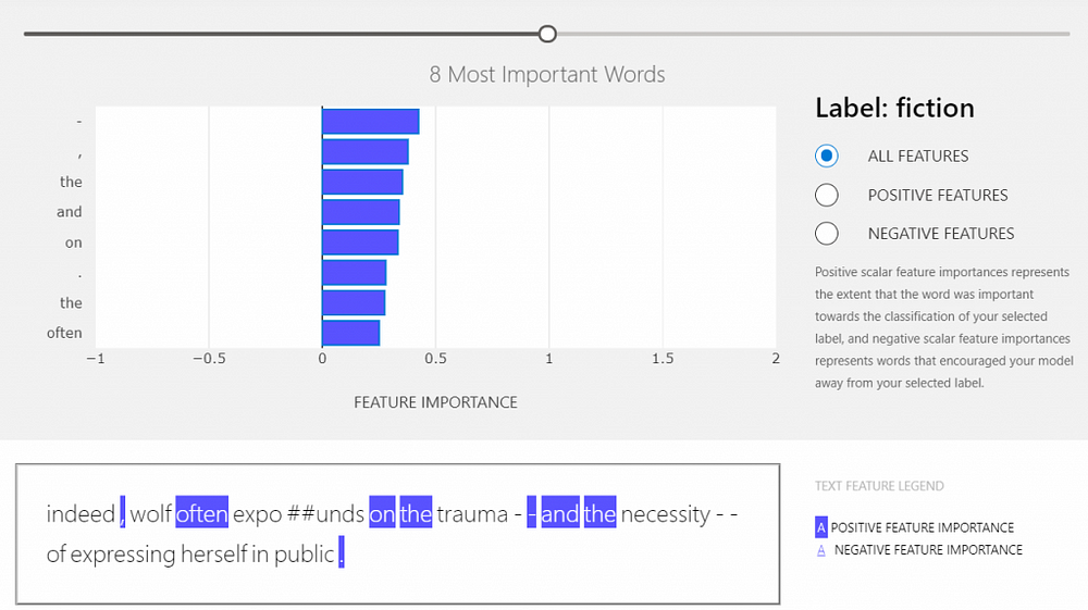
print(text, true_label, predicted_label)

explanation_unified = interpreter_unified.explain_local(text, true_label)

This result does not really provide an outstanding information, but it is possible to visualize which word has an impact on the prediction results, and which ones are not.

Dashboard

This is an interactive widget that shows whether the specific word has an effect on the prediction (positive features) or not (negative features). To generate and view this dashboard, run the following code.

from interpret_text.experimental.widget import ExplanationDashboard
ExplanationDashboard(explanation_unified)

With the slider on the top of the dashboard, the number of important features shown can be set. On the right side, the user can see the label given to the provided document. Under this, the user can choose to see all the features or only the positive or the negative ones. By hovering on the bars in the graph, the user can see the importance values.

Conclusion

In this post, users got the chance to pre-process the data, train a model that is able to predict the genre of a specific sentence, and explain how the pipeline works behind the scenes.

With the use of the Unified Information Explainer, users get a good overview of how the model uses the data that is provided, which allows them to improve the pipeline easier. In this post we learned about the explainer, built a training pipeline and after evaluation, generated a dashboard to understand, which words have an impact on the predicted label.

Continue the experimentation with other explainers:

• Classical Text Explainer
• Introspect Rationale Explainer

Contribution:

GitHub: Interpret-Text