In the last few years, artificial intelligence (AI) has become more and more prevalent and powerful. Many speeches around AI nowadays explain how these technologies can be beneficial in predicting stock prices and creating value for an organization. Even the online courses that are meant to educate newcomers in the field focus on the financial benefits of AI.
In today’s materialistic world, I would like to focus on how the very same technologies can be beneficial in predicting natural disasters and eventually increasing survival rates and improving quality of life.
The disasters caused by natural phenomena have been present all throughout human history; nevertheless, their consequences are greater each time. This tendency will not be reverted in the coming years; on the contrary, it is expected that natural disasters will increase in number and intensity due to global warming.
According to world statistics, the increase in the number of world disasters between the decades of 1987-1996 and 1997-2006 was 60% (going from 4,241 to 6,806), whereas the number of dead people during these periods increased a hundred percent (it went from more than 600,000 to more than 1,200,000). Source: Using Machine Learning for Extracting Information from Natural Disaster News Reports
More than nine million Australians have been impacted by a natural disaster or extreme weather event in the past 30 years. The number of people affected annually is expected to grow, as the intensity, and in some areas, the frequency of these events continue to grow. These costs include significant, and often long-term, social impacts, including death and injury, as well as impacts on employment, education, community networks, health, and well-being. Source: Natural Disasters in Australia
Humans have been trying to predict earthquakes at least since first-century China when they used this device: like a jar, with metal dragons facing each compass direction, and surrounded by frogs with their mouths open. If the ground shook somewhere in the region, the metal ball in the dragon’s mouth would drop out into the frog’s mouth, roughly indicating the direction of the earthquake. Many similar predictions actually sounded reasonable, but after some research, those things were concluded to be natural phenomena with little to no correlation to earthquakes. Source: 7 ways humans have tried to predict earthquakes
AI however relies solely on data.
Multiple researchers are creating their own applications to predict earthquakes and aftershocks. Moreover, these systems also monitor aging infrastructure. AI can detect deformations in structures, which can be used to reduce the damage caused by collapsing buildings and bridges, or subsiding roads.
In this article, you will read about a real-life example of saving more lives with Artificial Intelligence: how to examine a natural disaster, and how to use that observation to save more lives.
Nepal Earthquakes
In April 2015 there was an earthquake with 7.8 magnitude and an epicenter in the Gorkha District of Nepal. The disaster killed almost 9000 people and injured 22000. This horror was in most cases caused by the collapsed buildings in the earthquake.
Many data scientists have been working hard to improve the survival rate of the next earthquake. Our mission is to build a predictive machine learning model to investigate and understand the risks of damage in case of another natural disaster. The result of our findings is available for mitigation of which buildings might need strengthening before the next earthquake. By this not only the memorial buildings and homes could be saved, but also thousands of lives.
What is Data Science?
Data science is really just an umbrella term, it refers to figuring out ways to study and solve problems with data. To do that effectively, you need a range of skills: computer science, mathematics, statistics, and whatever domain you are in, you need expertise in that domain. For example, for this project, you might need to understand architecture and some kind of forecasting of natural disasters.
Data scientists are absolutely obsessed with data. The first thing we always do if we have a problem to solve is that we are looking around for all the possible data sources which we can bring to bear on this problem.
Now we have to figure out how to acquire the data, and how to get it into some system, such as a data warehouse, Databricks, or maybe Azure Machine Learning Studio.
But of course, the data is not always arriving in the shape we hoped for, so we might have to spend a lot of time on transformation, cleaning, re-shaping, and so on. Then we need to understand the relationships in the dataset, like, what is the data trying to tell us about the problem we are trying to solve, which of the features or variables actually seem to be useful, and which may just add noise to the situation.
Finally, we are going to do some predictive analytics or modeling, and through that, we hope to deliver value back to our customers or end-users, which helps them drive decisions and make them even better.
Machine Learning
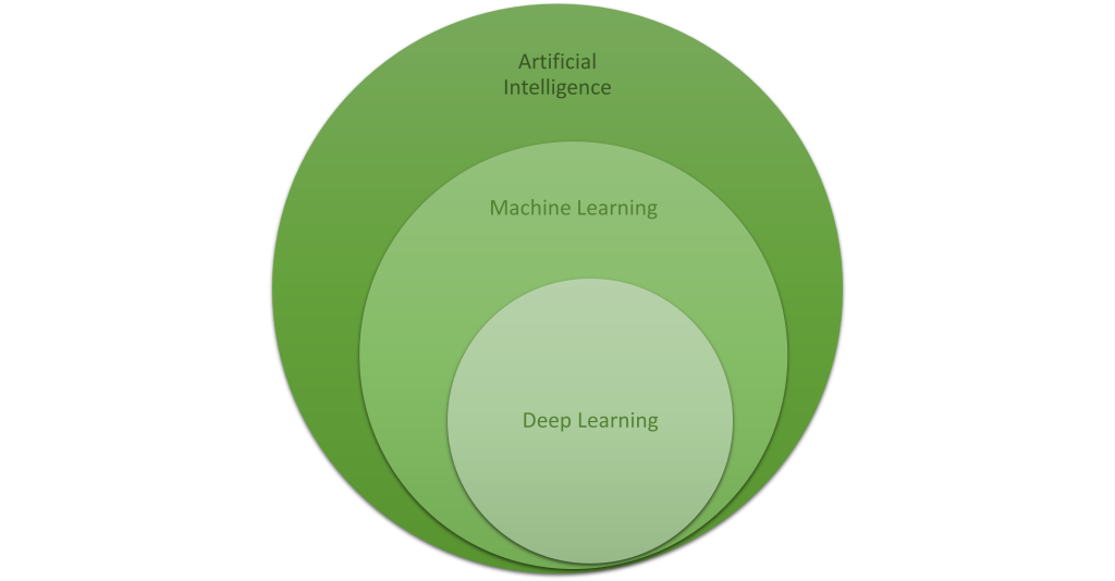
I often see confusion around the terms Machine Learning (ML) and AI. Let me clarify how these are connected to each other.
Artificial intelligence (AI) is a technique that enables computers to mimic human intelligence. It includes ML, which is a subset of AI. ML includes techniques such as deep learning which are neural networks that permit a machine to train itself. With ML techniques we can enable machines to improve at tasks with experience.
But how a machine can be trained?
Learning can be defined as “the process of knowledge acquisition. Humans learn differently, but all involve experience, While humans have the ability to reason, computers do not have that ability therefore they learn through algorithms.
Supervised learning generally includes a set of labels along with data, in here “the algorithm generates a function that maps inputs to desired outputs”. This learning type is commonly used for classification and regression problems, for instance, it can be used for classifying whether a building is in danger when another earthquake comes.
Unsupervised learning does not deal with labels, and only includes input data, meaning that the model has to find structure or patterns within the dataset itself. Common techniques include clustering and dimensionality reduction. Unsupervised learning techniques can be used for instance in speech recognition.
Reinforcement learning is “where the algorithm learns a policy of how to act given an observation of the world. Every action has some impact on the environment, and the environment provides feedback that guides the learning algorithm”. This technique is commonly used in autonomous driving or game development.
ML models generally have an iterative nature, involving four stages. Let me sketch up the main steps you need to take while working with an ML model:
Prepare data: We pull in the data into some system and prepare it for training. Data can come from various sources, generally speaking – in ML solutions-the more reliable data the better. Prepare data step involves data cleaning, data exploration, and splitting.
Exploration of the data helps developers understand the dataset and its structure. It is crucial to interpret what data is available and how it can be utilized for a model, this stage typically includes checking the data type and understanding different rows and columns within the dataset.
After the dataset is understood, irrelevant observations can be deleted as those would only add noise to the dataset. Typically, datasets include missing values and duplicates, whilst duplicates are generally get removed, to avoid a biased model, missing values are simply not understood by many algorithms.
and splitting (to train and test data, train data will be used to train the model, and we can also evaluate our model with the test data)
Train model: Training an ML model starts with choosing, which specific algorithm we want to configure our model with.
Raw data is transformed into features that the model can understand or in other words, feature engineering is done, which can include feature generation often used to make ML models more reliable.
After the goal of what the model will be used for is clear, available datasets are known together with the learning task the right algorithm must be selected. Typically, ML problems can be solved in many different ways, therefore, multiple solutions are usually developed and compared for the same problem to find the most feasible solution.
There are several approaches to each of these steps, but selecting the right algorithm is a rather complex task, Microsoft provides us with a cheat sheet that we can review before getting started.
Score model: this is the process of generating values based on a trained ML model. The generic term “score” is used, rather than “prediction,” because the scoring process can generate so many different types of values: a list of recommended items, numeric values, a predicted outcome, and so on, depending on what data you provide, and how you train the model.
Evaluate model: evaluation basically is metrics that tell you how well your model works, for example, the accuracy of a predictive model means how well it predicts the future.
This is a never-ending iteration process as when we find during evaluation that our model doesn’t work well enough, you would start over by reviewing the data, possibly further feature engineering and hyperparameter tuning to achieve better performance!
What we want to do is to build a predictive model which is able to answer our question, by learning from the data we provide: Which buildings are in danger when another earthquake comes?
Predictive analytics deals with designing statistical models or ML models that predict. These models are calibrated on past data or experience (features and labels), they learn from it to predict the future.
Azure ML Workspace
Teaching a machine might sound like some kind of black magic, but thanks to the tools provided by Microsoft, you have the chance to easily get started with learning about the different training algorithms, and then understand what the result tells you with the use of Azure Machine Learning.
This web experience brings together data science capabilities and ML assets into a single web pane that streamlines ML workflows. It is considered the top-level resource providing a centralized place to work with all the artifacts required to build a solution. The workspace keeps a history of all training runs, including logs, metrics, output, and snapshots of scripts.
Access ML for all skills to boost productivity
Rapidly build and deploy ML models using tools that meet your needs regardless of skill level.
Use the no-code designer to get started with ML or use built-in Jupyter notebooks for a code-first experience.
Accelerate model creation with the automated ML UI and access built-in feature engineering, algorithm selection, and a lot more features to develop high-accuracy models.
Operationalize at scale with robust MLOps
MLOps or DevOps for ML, streamlines the ML lifecycle, from building models to deployment and management.
Use ML pipelines to build repeatable workflows and use a rich model registry to track your assets.
Manage production workflows at scale using advanced alerts and automation capabilities.
Take advantage of built-in support for popular open-source tools and frameworks for model training and inferencing
Use familiar frameworks like PyTorch, TensorFlow, scikit-learn, and more
Choose the development tools that best meet your needs, including popular IDEs, Jupyter notebooks, and CLIs or languages like Python and R.
Build responsible AI solutions on a secure trusted platform
Access state-of-the-art technology for fairness and model transparency. Use model interpretability for explanations about predictions, to better understand model behavior.
Reduce model bias by applying common fairness metrics, that is automatically making comparisons and using recommended mitigations.
Enterprise-grade security with role-based access control, and virtual network support to protect your assets.
Audit trail, quota, and cost management capabilities for advanced governance and control.
An Azure ML Workspace is distributed into three components: Manage, Assets, and Authoring.
Manage
Compute
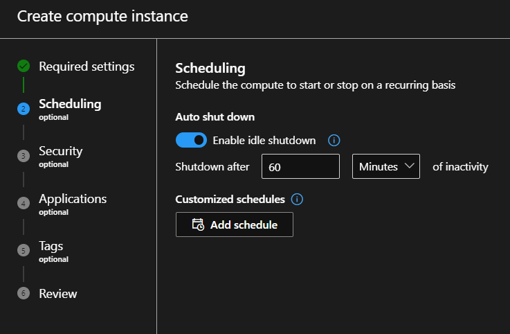
Create a new compute with a memory-optimized standard CPU. Provide a name, on the Scheduling tab, you can schedule start-up and shut-down times.
It is a good idea to shut it down when inactive, so it won’t charge you if you forget to switch it off yourself.
Monitoring
Monitor your models to get alerted in changes to data drift as your model is in deployment.
Data Labeling
You can create labeling projects with image classification or object detection here. From here, you can also manage labeling workflows, scale-out labeling efforts to multiple labelers, and leverage the power of ML to improve speed and accuracy with ML Assist.
Linked Services
You can connect different Azure services to your Azure ML Workspace, for example, a Synapse workspace.
Assets
Data
Here you can import data into the workspace, so it is available to use for your pipelines. You can upload the data from your own PC, Azure storage, SQL databases, a web file, or Azure Open Datasets, these physically are stored in Azure Storage that is deployed together with the workspace. These datasets are versioned, so you can easily monitor the changes in the data. You can set up dataset monitoring to detect data drift between the training dataset and inference data. Azure ML also allows you to set up scheduled data imports even from external sources including Snowflake DB, Amazon S3, and Azure SQL DB.
Jobs
When we run something within the workspace, those runs can be monitored here.
Components
Here you will find your custom components created as building blocks for your ml projects, which is a self-contained piece of code that does one step in an ML pipeline. Components are the building blocks of advanced ML pipelines. Components can do tasks such as data processing, model training, model scoring, and so on.
Pipelines
This is where you can see the available pipelines for your jobs, these can be triggered from connected services too, eg. Synapse.
Environments
There are different setups that contain several already installed packages, rest assured you will find your favorite ones here too: Scikit-learn, TensorFlow, and more.
Models
Deployed and registered models are visible here. You can generate a Responsible AI dashboard for your models that provides a single dashboard to help you debug and assess your ML models’ fairness, errors, explainability, and more.
Endpoints
You can create real-time or batch endpoints for your deployed models.
Author
Notebooks: Understand data
Azure ML Notebooks is a fully managed cloud-based code-first environment for data scientists to author models, transform, and prepare data with Python or R. You can also build Automated ML (AutoML) experiments from the notebooks. You can create bash, text, and Yaml files here, which enables you to build an end-to-end pipeline for your scenario. They are pre-configured with up-to-date ML packages, GPU drivers, and everything data scientists need to save time on setup tasks.
To demonstrate how Notebooks works, let’s have a first view at the data provided by The Central Bureau of Statistics, they collected the largest dataset, which contains valuable information about numerous properties (area, age, demographic statistics, and more) of buildings that have collapsed in earthquakes in Nepal. Download the data from here.
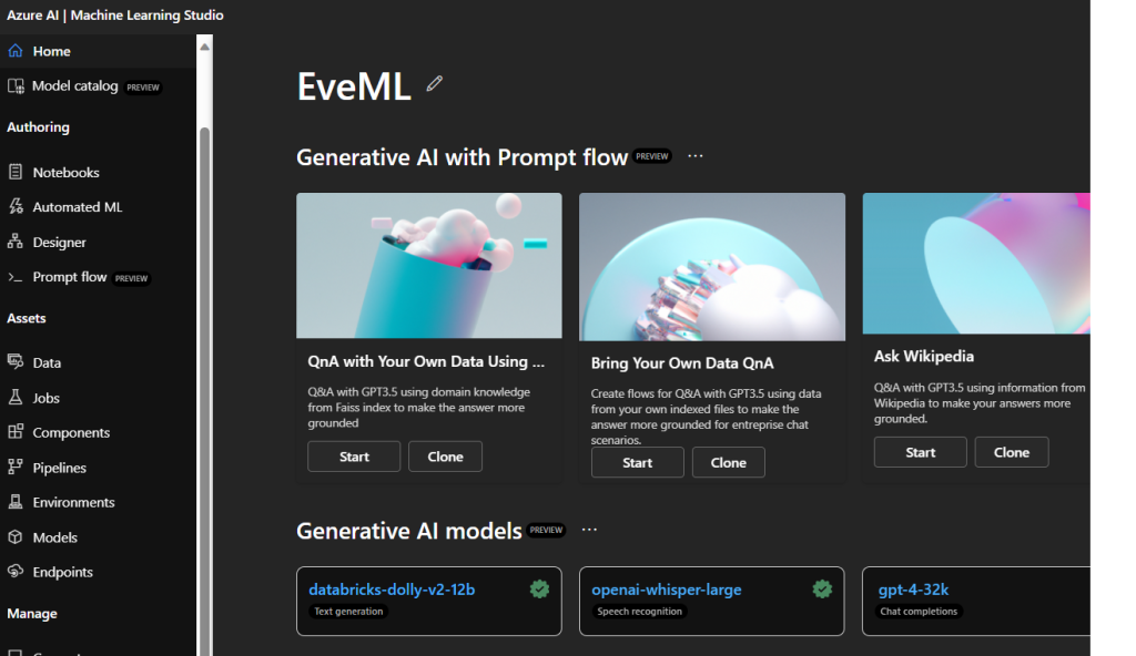
Create a new Azure Machine Learning Workspace and when the deployment is done, go to the resource and click on the Launch Studio button on the Overview page. You should see a panel on the left with the Notebooks, AutoML, and Designer options.
Start the Notebooks.
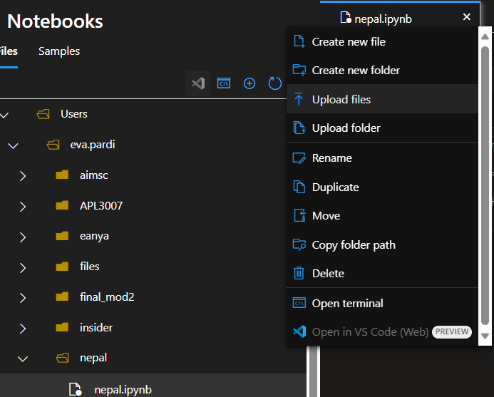
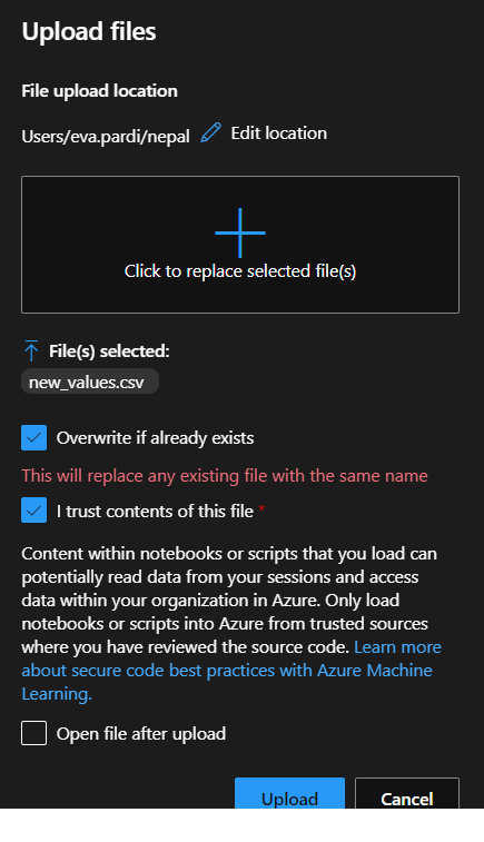
The folder structure is on the left, here you can create new files and folders. From the Samples tab, you can import a project built by Microsoft, to get started. Let’s start by loading the data from the folder you downloaded the files from GitHub. Hover over the folder where you want to place your files, click the three dots, and choose the Upload files option.
Select the new_values.csv from the new_values folder and click on the Upload button.
Let’s also create an IPython Notebook, by hovering over the folder and clicking on the three dots, then clicking on the Create new file option. Make sure, the file type is .ipynb, provide a name, then click Create. The compute can be created from here as well, it will be used for running our code. To create one, you can press the + sign next to Compute on the top of the notebook, or at the icon in the bottom left side of the menu. Specify the kernel on the right side, for this article, I use Python 3.10 – SDK v2.
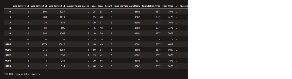
Pandas stands for “Python Data Analysis Library”, it has a lot of great functions to use on objects called dataframes. Dataframes are interactive tables, which you can easily manipulate and transform. First, we will use
import pandas as pd
dfValues = pd.read_csv("new_values.csv")
dfValues
After displaying the data, we can see how many columns and rows we have in our dataset, and you also get an overview of the stored values.
Also, we can get the type of each column using this code:
dfValues.dtypes
The field of statistics is often misunderstood, but it plays an essential role in our everyday lives. Statistics, done correctly, allows us to extract knowledge from the complex, and difficult real world. A clear understanding of statistics and the meanings of various statistical measures is important to distinguish between truth and misdirection.
When we have a set of observations, it is useful to summarize features of our data into a single statement called a descriptive statistic. As their name suggests, descriptive statistics describe the quality of the data they summarize. It is useful when you have so much data to observe what we have here, and instead of scrolling through and trying to understand just by looking at it, we can use some nice Python functions.
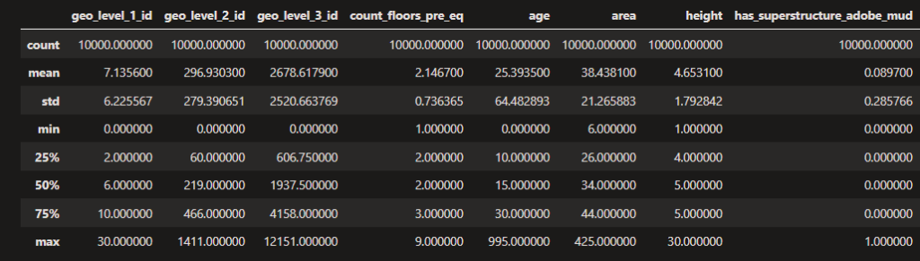
dfValues.describe()
What we can see here in the first row that how many not-null values are in the column (as Python’s describe() function counts only the not empty fields), and by this information we can be sure that each of the rows in each of the observed columns hold not-null values. This is important, otherwise it gives a lot of noise into any calculations and predictions.
Have you also noticed the number of columns of the results? The describe() function returns information only about the numerical columns, and removes the other types from the observation. For simplicity, we are not going to discuss how string features are used during modelling.
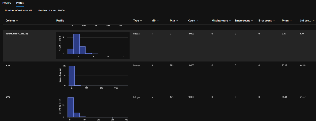
Another observation you can make here is the min and the max values for each column. For example, the buildings have minimum 1 and maximum 9 floors, or that the age of the building is at least 0 and can go up to 995.
Another important observation is at the columns starting with has_, that it’s minimum is 0, and the maximum is 1. I could assume, that these are probably true or false, but I cannot be sure about it right now. We can make a check on for example this has_superstructure_adobe_mud column with the use of the unique function.
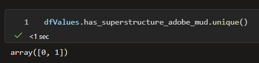
dfValues.has_superstructure_adobe_mud.unique()
This shows the distinct values of the chosen column, so now we are sure, that these columns hold true and false values.
Descriptive statistics fall into two general categories: the measures of central tendency and the measures of spread. As we have used the describe() function, now we have some important statistics for the dataset.
The mean is a descriptive statistic (falls into the central tendency category) that looks at the average value of that specific column. The measures of spread (also known as dispersion) answer the question, “How much does my data vary?”
The standard deviation is also a measure of the spread of your observations but is a statement of how much your data deviates from a typical data point. That is to say, the standard deviation summarizes how much your data differs from the mean.
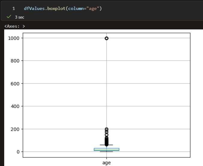
For standard deviation, we can also use a visualization tool – just in case, to have a graphical overview of the data. For example, let’s observe the age.
dfValues.boxplot(column="age")
In the case of the age we can see the mean as a blue box, and that most of the buildings are between 0 and 200 years, which are very close to the mean, and there are some outlier values, with around 995 years – which are probably memorial buildings that have collapsed in the earthquake.
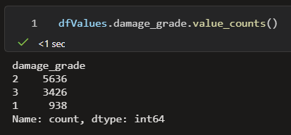
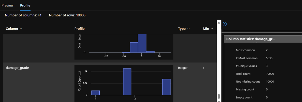
The label column is the damage_grade, which indicates how high is the risk of damage for the buildings in case of another earthquake (1 – low, 2 – medium, 3 – high). So our model is going to predict the risk by learning from “experience” data. We can further investigate the label column, by running the following code.
df.damage_grade.value_counts()
You can see that there are 3 different values in the damage_grade column, and also the number of features that are available for each of the labels. The best case would be if these numbers were quite close to each other, though it is visible that the number 2 has many more examples than the labels 1 and 3. This is a problem because if the model is trained on more examples with label 2, it more often returns label 2 even when the risk is supposed to be high or low. We shouldn’t train the model on unbalanced data, so we are going to deal with this issue when we start the transformation and preparation of the data before training.
When we prepare for the work with the predictive model, we can already have a good understanding of which features we keep, and which ones we leave out. For now, we can conclude the information we learned with statistics and some investigations. If you want to learn more about your data, create a profiled dataset.
count_floors_pre_eq (int): number of floors in the building before the earthquake. When two buildings are the same height, the one with fewer floors has a higher damage risk because the construction is weaker than another one that has more floors.
count_families (float): number of families that live in the building.
has_secondary_use (binary): indicates if the building was used for a secondary purpose
square (float): square root of the area
difference (float): the difference between the square root of the area and the height of the buildings
The next 10 features indicate which material was used for building the superstructure. The first one is the weakest with a high risk of damage, and the last one is the strongest with a low risk of damage.
has_superstructure_bamboo (binary): Bamboo
has_superstructure_mber (binary): Timber
has_superstructure_adobe_mud (binary): Adobe/Mud
has_superstructure_mud_mortar_stone (binary): Mud Mortar – Stone
has_superstructure_stone_flag (binary): Stone
has_superstructure_cement_mortar_stone (binary): Cement Mortar – Stone
This is all nothing, you can even write your own ML models and data science tasks here in the Notebooks. You can create and deploy models, and automated workflows and you can also create an automated ML run.
For POC you have to provide results quickly, instead of building data-wrangling actions, and predictive ML models from scratch, let me show you how the next tool in Azure ML Workspace can support your presales or POC work.
Designer: Data preparation, training, deployment
Do you also have the situation when the manager walks up to you and asks: “How long time do you need to build an ML model?” After some questions are asked, you will receive data and conclude the aim of the model. A first step from here could be to put together a POC that shows the analytical workflow and allows easier estimation of development time.
Data scientists can use a rich set of built-in components for data transformation and preparation, feature engineering, model training, scoring, and evaluation. ML experts can visually craft their complex end-to-end ML training pipelines with their own code. ML engineers can construct the operations pipeline in a similar drag-and-drop approach. Azure ML Designer visualizes complex ML training pipelines and simplifies the process of building-, and testing models and operation tasks by bringing built-in components, data visualization, model evaluation, and MLOps (DevOps for ML) integration. It enables users to automatically generate scoring files, register models, and build images using Azure Kubernetes Service (AKS) for scale. The cloud-based asset also provides users with a set of built-in algorithms, feature engineering, and model evaluation to further simplify and dramatically accelerate the process of building ML solutions.
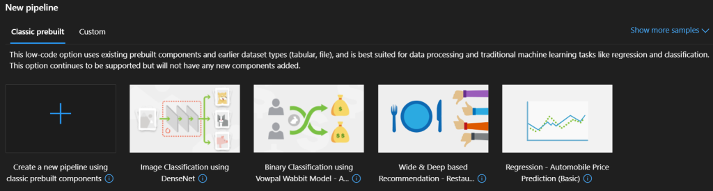
From the welcome screen of the workspace, start the Designer. Note that you can try out already generated sample pipelines to get started.
Click on Create a new pipeline using classic prebuilt components. This environment is really similar to the old Studio, but numerous new features are added, like pre-trained models for anomaly detection or computer vision and so on. You can drag and drop the components into your canvas and when you submit the pipeline for run, you can review the results in the Jobs asset.
Data transformation
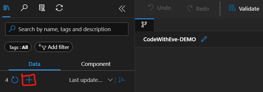
Let’s upload the dataset that we used in the previous section with the plus sign.
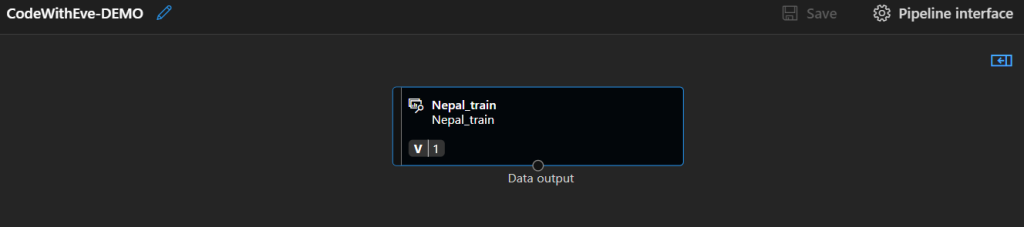
Give it a name, and choose Tabular as the data type. On the next tab, choose to upload from local files, and leave the destination as default. Upload the new_values.csv, then leave the rest of the settings as is, review the data, and click Create. This dataset is stored in a Storage Account, which was provisioned together with your workspace. Pull in the uploaded dataset to the authoring area, and then right-click on the component to Preview data.
If you click on the Profile tab, we can see some visualization showing an analytical overview of our unbalanced dataset, additionally, some information we learned in the Notebooks with the describe() function.
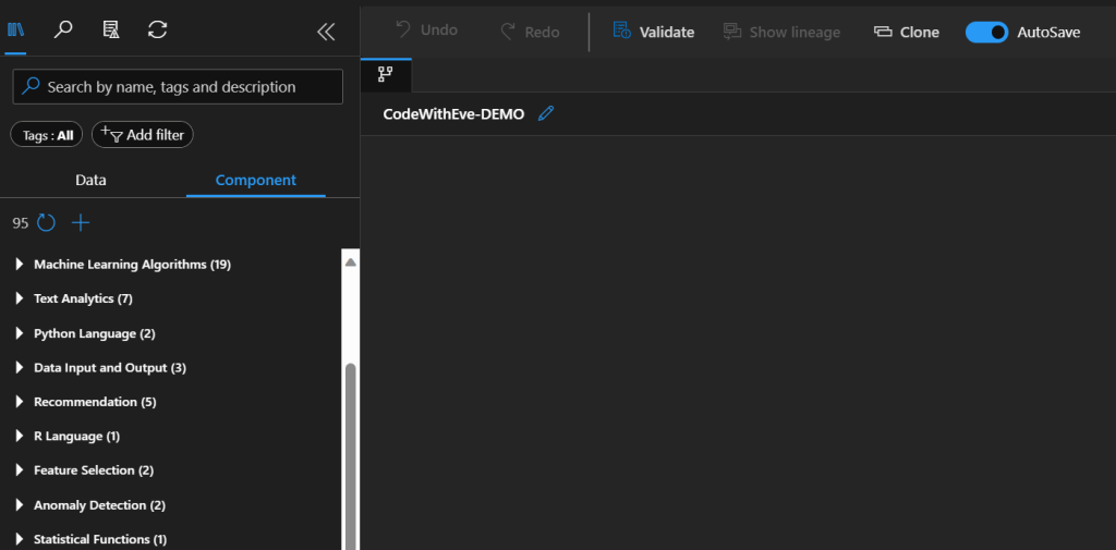
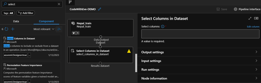
To exclude noisy values (such as non-numerical columns that were not shown in the describe function’s result), we can use the Select Columns in Dataset component. In the left panel choose the Components tab and search for the component. After you drag and drop the component to the authoring area, connect the dataset to the component. Click on the component twice to open the parameters window, and click Edit columns.
A new window opens, put in the following list, and press Enter, then click Save.
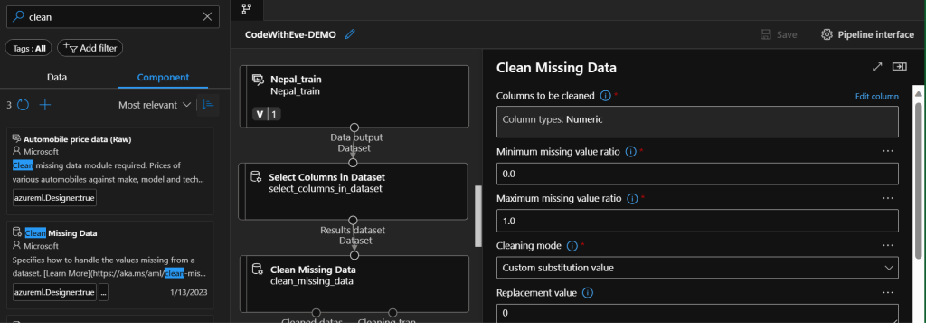
Even though we know that we do not have empty fields, I would like to show another important component, the Clean missing data, which can exclude or transform all rows with missing values. Why do we need to choose first the relevant columns and then exclude null values instead of the other way around? Imagine that there are missing values in the columns which we would exclude anyway. If we first remove the entire row because of that missing value, we could exclude maybe useful features. So, therefore we first must include only the useful features, and then remove the possible null values. Instead of removing rows, I will just choose to use a custom value and replace the empty values with 0 – this only works on numerical columns. Drag and drop the Clean Missing Data component, double-click on it, then on the left side, click Edit columns, and choose Numeric Column types to operate on. In the Cleaning mode, choose Custom substitution value, and as Replacement value write 0.
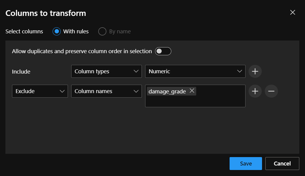
Another important step of data preparation is called Normalization, to exclude outlier values like we have seen for example at the age column. The goal of normalization is also to change the values of numeric columns in the dataset to use a common scale, without distorting differences or losing information. This is useful since most of the columns have different metrics with different scales, now all the numerical columns will be on the same range of values. The component we use is called Normalize Data, the transformation method I chose is ZScore, and the Columns to transform are all numerical columns except the damage_grade.
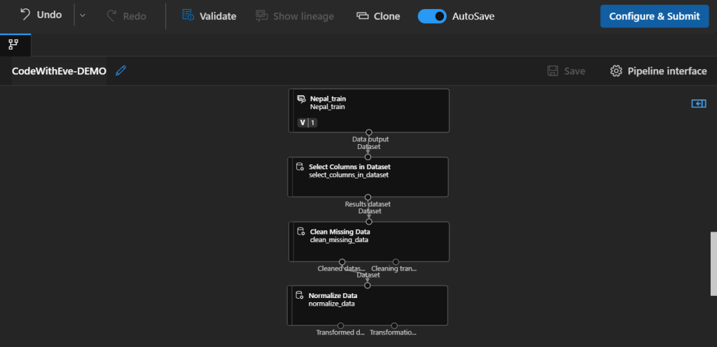
ZScore uses the mean and the standard deviation for calculating each value. It takes the value and decreases it with the mean of it, and then divides it with the standard deviation of it. This is how your pipeline should look now:
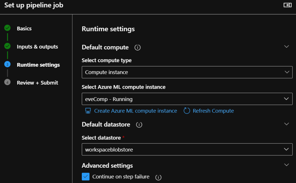
Let’s make our pipeline runnable! Click on Configure & Submit. On the Basics tab, provide a name for the experiment, then click Next. On the Runtime settings tab choose the compute instance that you used with the Notebook and click Next. After reviewing your settings, click Submit.
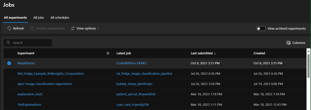
The job is now submitted, and you can monitor it by clicking on the Jobs asset in the left panel menu.
Over sampling
The challenge of working with imbalanced datasets in most ML techniques is ignored, and in turn have a poor performance. Although if you think about it, typically the performance on the minority class is also very important. In our case the high risk of damage is a minority class for example. I’m using the SMOTE approach to solve this issue with oversampling and with the help of this technic I can provide the model close to equal number of samples for the labels.
Note, that there are a lot of features for the level 2, and a very low amount for the level 1 and 3 damage_grade. The component only works with two categories at once, but I have a great workaround for you.
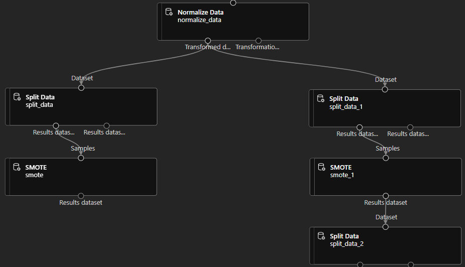
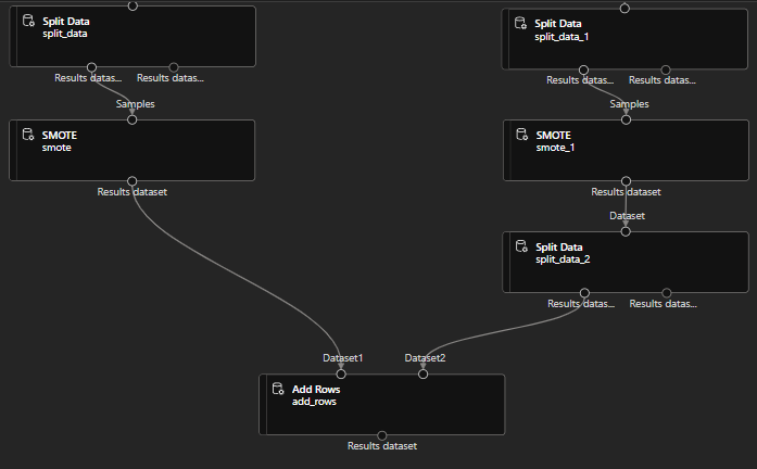
First we are going to split the data twice with Relative expressions. Use Split Data components on both sides and choose Relative Expression as splitting mode. On the left we want only the level 1 and 2, on the right only level 2 and 3, because we are going to compare the level 1 and 3 features to the level 2.
Code for the left side: \”damage_grade” < 3 right side: \”damage_grade” > 1
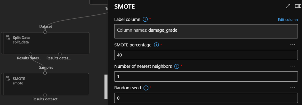
Now let’s get the SMOTE components, and choose the damage_grade column to operate on, then set the percentage like on the picture below. The percentage specifies how much more features should be generated from a level, to align with the others.
Percentage on left side: 400 right side: 40
Remember, we have now two dataset, one of them includes damage_grade 1 and 2, the other includes 2 and 3, we have to put these together. For this we are going to use Split Data on the right with Relative Expression: \”damage_grade” > 2. The model now should look something like this:
Let’s use the Add Rows component, and from the right side we pull in the damage_grade 1 and 2, but from the other side we only need the 3, otherwise the labels would be biased again: 1, 2, 2, 3. So this is now the pipeline you should also see:
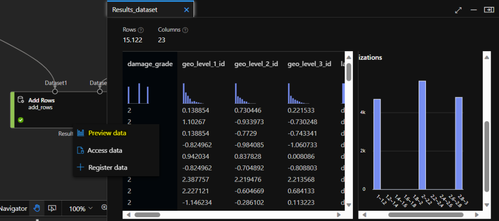
So Let’s submit this updated pipeline with the Configure & Submit button, and review the results. On the job view, right click on the Add Rows component and choose to review the result dataset. Note that the damage_grade column is now holding a much more balanced data.
Training
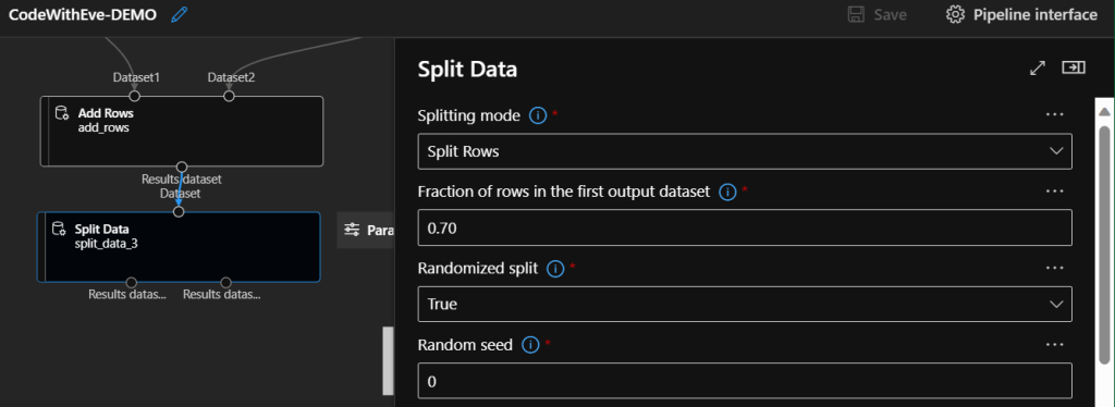
Now finally, with the help of the Split data component, we will prepare data for training and for validating the model. I set the fraction of splitting to 0.7, in which case 70% will be train data and 30% will be used to validate the model.
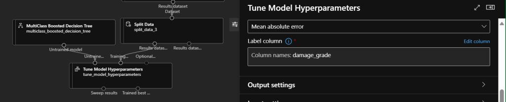
Now we are ready to train our model. For this we need to choose the best fitting algorithm. There are several specific types of supervised learning that are represented within the Designer, for example: classification, regression, or anomaly detection. When you are not entirely sure which algorithm works better for your specific dataset, you can investigate that by pulling in two – or more – algorithms in the same time. I chose a Classification model which is used when a category needs to be defined – like in our case with the damage_grade. Since we have more than two categories, we need to find a best fitting Multiclass Classification algorithm. Find suggestions in the cheat sheet provided by Microsoft. After thorough investigation, in my case, the best fitting algorithm was the Multiclass Boosted Decision Tree. During training we can use the Tune Model Hyperparameters, so the best fitting parameters will be defined and used for the iteration, to reach better prediction results.
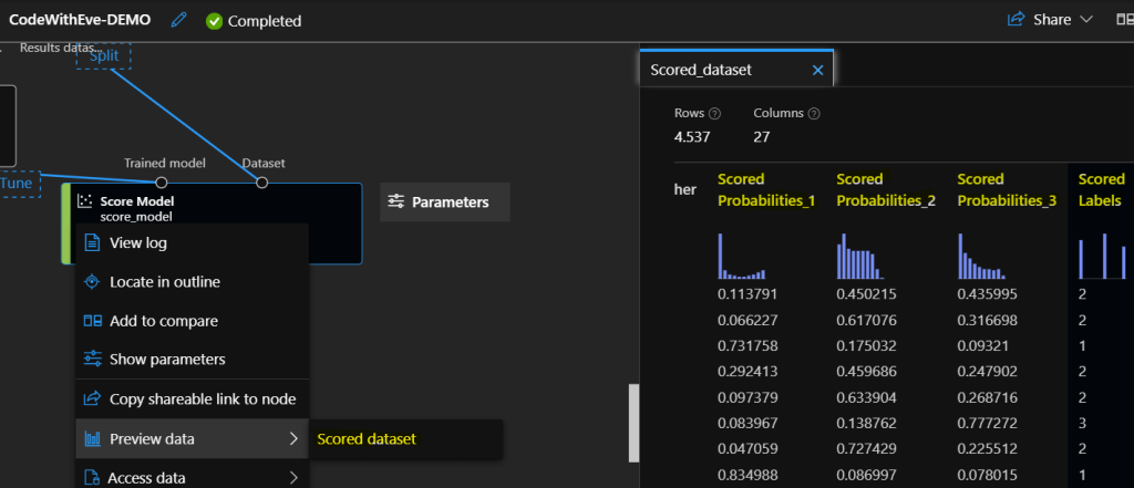
Scoring the model means, that it does the prediction. Use the Score model component for this, and connect the Trained best model output of the Tune Model Hyperparameters component and as Dataset, pass the second output of the Split Data component. Submit the pipeline, and let’s visualize the results. On the Job overview, right click on Score Model component, and choose to preview the Scored dataset. It shows the chosen damage_grade for a specific building, and the confidentiality of choosing the specific categories, in the last four columns.
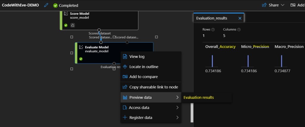
Evaluation is an essential step while building ML models, it tells us how well our model works. Let’s use the Evaluate model component for this task.
Accuracy refers to the average model-performance involves root mean square error (RMSE), which is the standard deviation of the errors in the prediction and mean absolute error, (MAE), the errors between paired observation calculations
Precision is a measure of goodness that determines the proportion of label items from the available ones. In short precision is one of the most commonly used evaluation metrics show the percentage of accurate recommendations.
Thanks to all these built-in components, you can quickly build an experiment, and find out by incremental trials, which setup works best for your scenario. When you are happy with the model, it can be deployed and used in production too. Deployment and usage of pipelines are discussed in another article. If you don’t want to spend your time on figuring out the best fitting algorithm for your scenario, maybe you want to look at the next section.
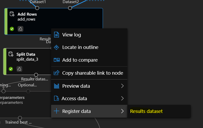
Before doing so, let’s register the clean and non-biased dataset in the environment. On the Job view, right click on the Add Rows component, and click Register data.
Provide a name for your dataset, and choose Tabular as data asset type.
Automated ML
If you are unsure which model fits best your dataset or solution, the no-code UI of Automated ML is the first you should try out. It allows you to easily create accurate models customized to your dataset and refined by different algorithms (deep learning for classification, time series forecasting, text analytics, image processing) and hyperparameters. You can increase productivity with easy data exploration and profiling with intelligent feature engineering. You can simply download the best model and improve it on your own PC too, and by pressing the Deploy button, your model is ready to be used from an API endpoint. And last but not least, you can build responsible AI solutions with model interpretability, and fine-tune your models to improve accuracy.
The Automated Machine Learning (AutoML) SDK allows you to run Deep learning solutions for Classification, Regression, Text Classification with BERT (on GPU) and Time series forecasting with ForecastTCN & HyperDrive.
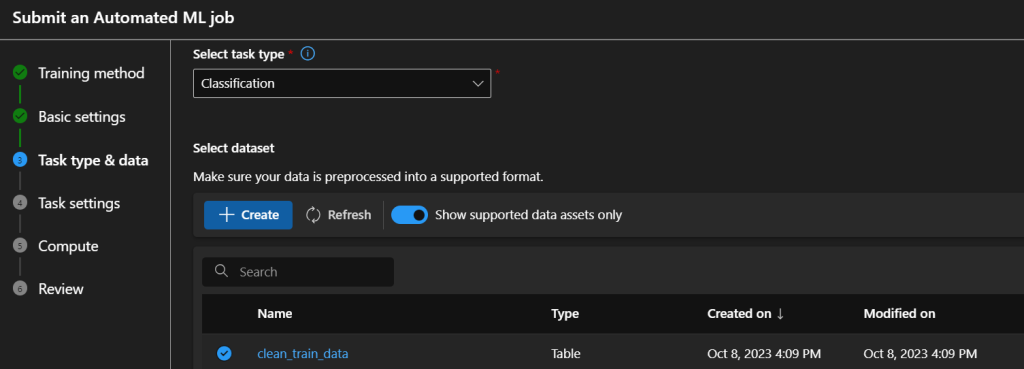
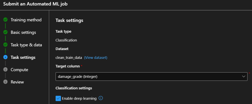
As I mentioned before, the UI is quite understandable, we just go ahead and create a new run. Start the Automated ML from the welcome page, and click New Automated ML job. On the Basics tab, you need to create a new experiment and provide a name for it. On the next tab we specify the algorithm type (Classification) and the exact same dataset as we registered in the previous section.
On the Task settings tab, we specify the label column (damage_grade) and you can enable deep learning (this setting requires a GPU compute that you should create and/or start on the compute menu before you come here).
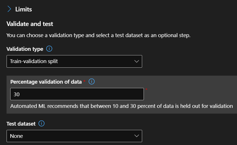
Here you can also specify a test data for your AutoML run, or define how many rows should be used for validation.
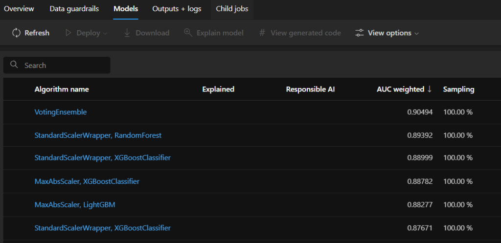
On the next window, specify the compute the job should run on (you can also try the serverless GPU option), and after reviewing your settings, submit the job. After initializing the run, we can observe the models that have been tried on the Models tab. The one on the top has the best accuracy.
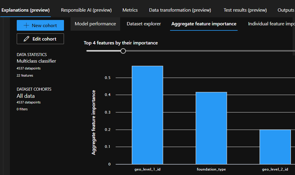
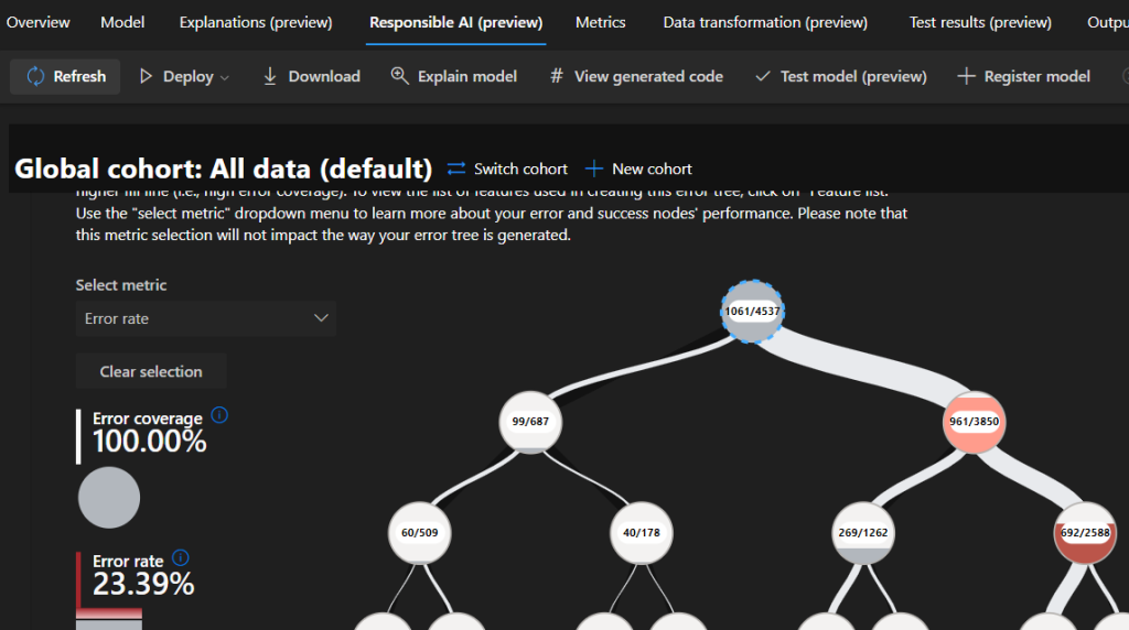
Click on the name of the algorithm and observe the top menu. You can easily deploy the chosen model as well by simply clicking on the Deploy button. We can download the code from here, and further improvements can be applied to it before deploying the model. You can create an explanation dashboard for your model by clicking on the Explain model button, for which you can choose the same compute instance as we used in the previous sections, and click Create. After the job has finished running, you can review the dashboard on the Explanations (interpretability) and Responsible AI tab:
On the Explanations tab, you can review the feature importance (what are the important features for the specific training run, what are the features that have the highest effect on the end result), and how the model performed on the data provided.
On the Responsible AI tab, in addition to what you can review on the Explanations tab, you can also see a detailed error analysis, and you can create dependence plots for the important features.
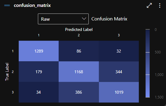
If you want to learn more about your model, you could take a look at the Metrics tab, where you can visualize all kinds of details. For example, my favorite is the confusion matrix, which tells us how well the model was able to define the specific damage_grade, or how confused is the model.
For example, the middle blue box shows 1168. This means that in 1168 cases, the model correctly predicted the label “2” (medium risk of damage) for buildings. The darkest box with 34 in it shows that it predicted label “1” (low risk of damage) 34 times for buildings when they actually have a high risk of damage, label “3”.
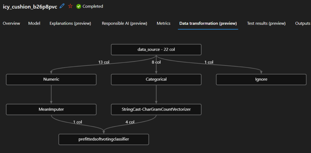
If you want to learn more about how your data has been transformed, you can see that in the Data transformation tab.
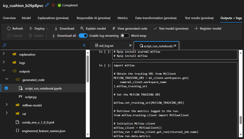
If you have provided test data for the AutoML run, you can also review the test results on the next tab. At the Outputs + Logs tab, you can find everything in the same place, the code, the scripts, and files needed for deployment, or further development.
Azure ML Workspace can be used for simple and complex problems as well, as for code-first and no-code scenarios. I think it is a great place to get started with understanding ML, and learning about the algorithms and the flow of training.
The best choice of algorithms and data features are highly dependent on what problem you try to solve, and what kind of dataset you have.
And remember, spend as much time as possible with feature engineering, because that has the biggest impact on the accuracy of the model. Training and testing the model helps you to see where the model needs to be improved to get better accuracy of prediction. Iterative improvements are key to ML modeling and the best result is the aim – this is the reason, I think, why Artificial Intelligence is an always improving field.